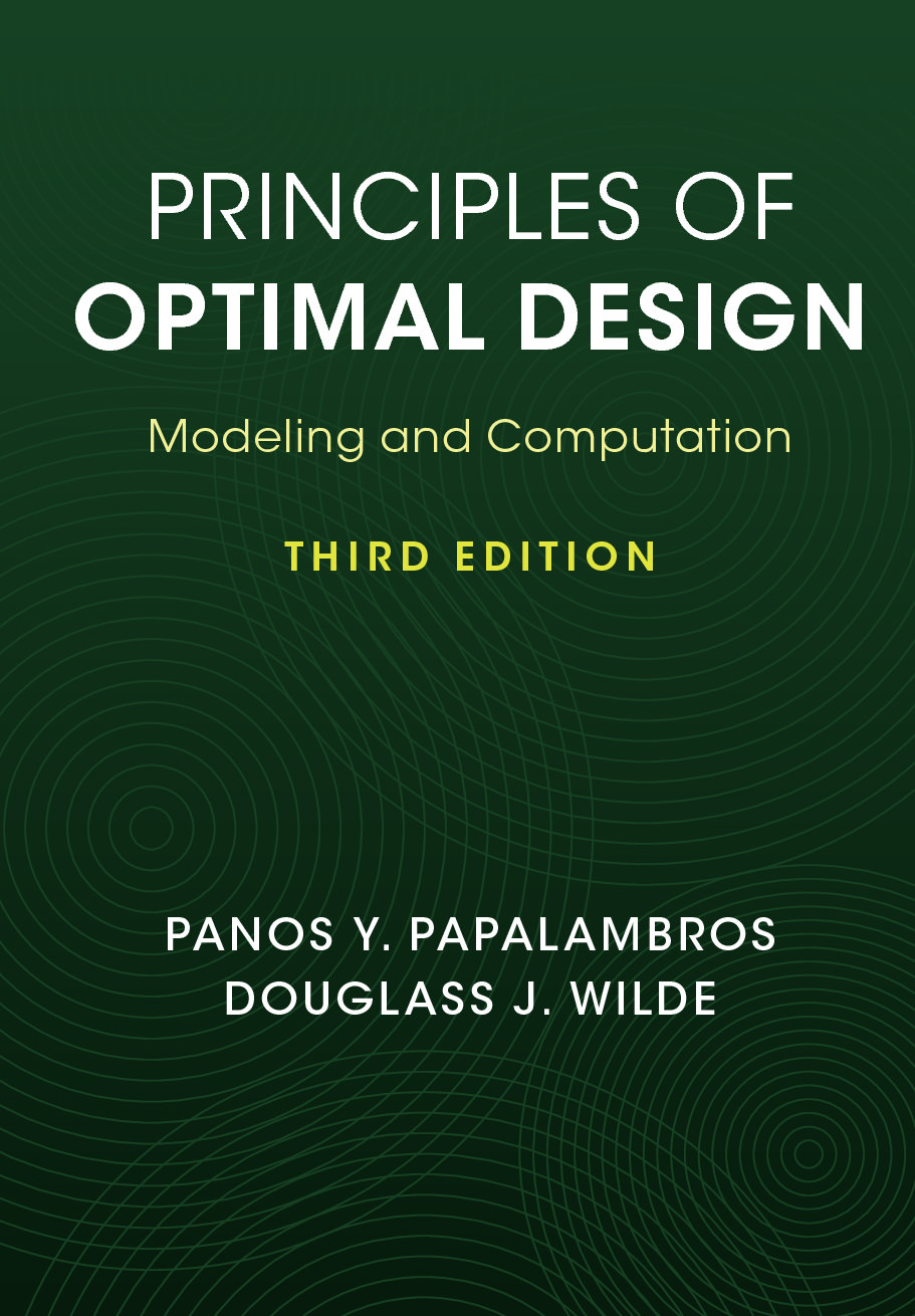
From the author:
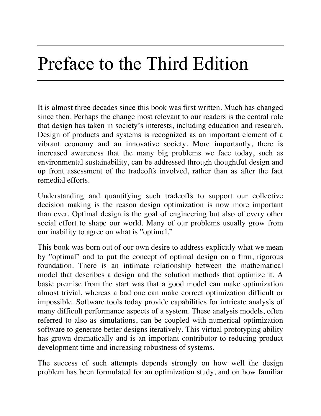
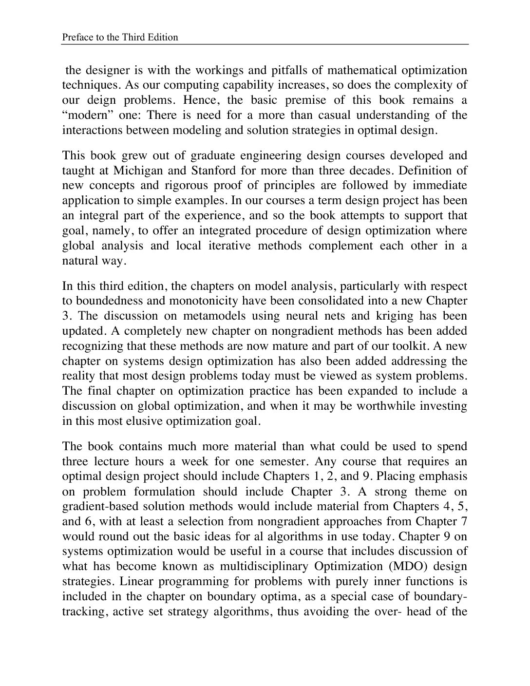
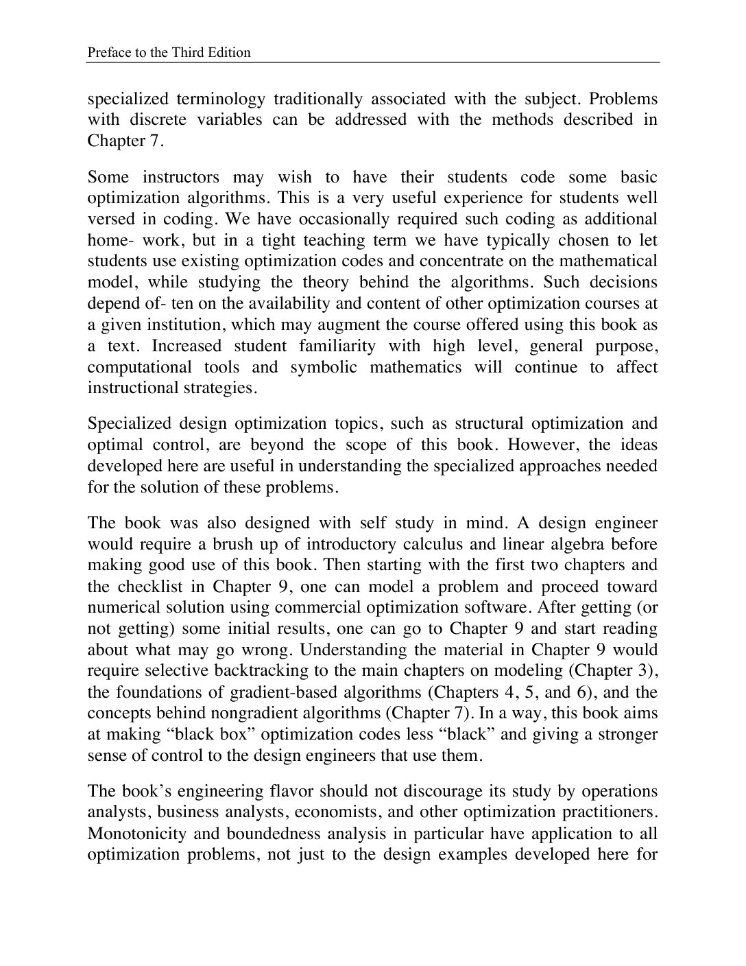
The book was conceived and written in the mid 1980s to highlight the interplay between the mathematical modeling of design as a decision-making problem and the computational algorithms that will allow the practitioner to solve these problems successfully. Since then, design optimization has become ubiquitous in industry. New classes of algorithms have been developed. Problem complexity has increased and system design has become more critical. Excellent software tools are widely available and take away a lot of the labor. I wanted the new edition to capture these developments and hopefully to maintain its value to the design practitioner. Moreover, I wanted to show that the original motivation for the book is still valid today just as much as it was thirty odd years ago.
Who is the primary audience for this book?
Mathematical design optimization is a natural tool for practicing design engineers who work extensively with simulation-based design software. The mathematical nature of optimization is sometimes a deterrent and I tried to lower the burden and focus on developing a way of thinking. Advanced seniors and graduate students in engineering who plan to work in advanced product and process development are the obvious immediate audience.
What are the market needs/key challenges this audience faces?
The math content can be daunting at first sight. However, if you persist a bit, you find that what you really need is very basic calculus and linear algebra at the freshman or sophomore levels in engineering schools. Actually, once you accept the math need, you realize that those old abstract concepts are practical tools that give you lots of insights. Some of the newer modeling and nongradient methods require more advanced statistics than most people in that group will likely know. But if you miss some of the details, you will still get the thinking behind the methods and will be wiser in using them.
Does the book solve this need/challenge? How?
When practical, we have included simple examples to illustrate each math idea and interpret it in a design context. Sometimes you have to write your own code to “get it” and I have included some suggestions, as students are increasingly facile with coding. The exercises are also meant to help hone this understanding. The last chapter on “Principles and Practice” takes a longer view of how all this math will work in practice —or not work! We also have there a detailed checklist containing all the steps you should take throughout a design optimization project, from setting up the problem to interpreting the numerical output of algorithms.
What unique features do you think make the book stand out in the market?
It’s just the key idea that the problem model and the solution strategy in design optimization are intricately coupled. Each informs the other and leads you to success — or controlled failure so you can try again. The other key point is to honor the math needed but keep it at the lowest level possible. Finally, I hope the price is low enough to make it stand out – following an understanding with Cambridge University Press dating to the first edition.
Key Chapters In The Book
1. Optimization Models
We define the design optimization problem and associated jargon, and describe most of the properties and issues that occupy the rest of the book. We outline the limitations of our approach and caution that an “optimum” design should be perceived as such only within the scope of the mathematical model describing it and the inevitable subjective judgment of the modeler.
2. Model Construction
We discuss basic techniques on creating mathematical optimization models using metamodels, from the more classical forms of curve fitting to the newer ideas of neural networks and kriging. We provide detailed examples of constructing design optimization models, primarily to help the reader through an initial modeling effort.
3. Model Boundedness
In modeling an optimization problem, the easiest and most common mistake is to leave something out. This chapter shows how to reduce such omissions by systematically checking the model before trying to compute with it. Such a preliminary study often leads to a simpler and more clearly understandable model with fewer variables and constraints than the original one. The methods of this chapter, are informally referred to as boundedness analysis. At the same time, one should be cautious about the limitations of boundedness arguments because they are based on necessary conditions, namely mathematical truths that hold assuming an optimal solution exists. Such existence, derived from sufficient conditions, is not always easy to prove.
4. Interior Optima
We describe the differential (gradient-based) optimization theory for unconstrained problems with functions that possess derivatives. We derive necessary and sufficient conditions and then develop basic numerical algorithms based on these conditions that can be used to solve unconstrained problems.
5. Boundary Optima
We study problems where there are constraints and the function has a minimum at the boundary. Design models will often have boundary optima because of frequent monotonic behavior of the objective function. The differential optimization theory is extended to such constrained problems and the derived optimality conditions lead to basic computational methods for identifying constrained optima.
6. Local Computation
Numerical methods for solving optimization problems can fail for a variety of reasons. No single method exists for solving the general optimization problem with complete reliability. The chapter gives an appreciation of what is involved in designing algorithms and describes a small number of powerful methods that are generally accepted as preferable for design problems. The mathematical content aims to provide insight for the fine-tuning and coaxing that is often necessary for solving practical design problems.
7. Nongradient Search
We organize the discussion of nongradient methods in three parts, direct search methods, heuristic methods, and black-box methods. Direct search methods rely on ranking the objective function values rather than using the objective values themselves. Heuristic methods use some random process to generate new candidate solutions, and so the iteration paths and even the solutions obtained can change each time we perform a search. Black-box methods deal with problems that have no known model function structure that we can exploit. For example, functions generated by simulations have no discernible mathematical properties (like convexity), and so we refer to them as black-box functions. In this sense, all nongradient methods can be used for black-box problems. The two black-box methods described in this chapter were created to address design problems with expensive simulations, and so their main goal is to find an optimum quickly with few function evaluations.
8. Systems Design
System optimization uses partitioning and coordination to implement the basic principle of decomposition: Break the problem into simpler problem pieces (subproblems), solve each subproblem separately, and coordinate the subproblem solutions so that you can obtain the solution to the original problem. Decomposition-based optimization is useful if (i) the effort for partitioning, subproblem solution, and coordination is less than the effort required to solve the original problem; or (ii) the original problem is simply not solvable without decomposition; and (iii) the decomposition-based solution is indeed the same as the solution to the original non-partitioned problem. We discuss how to represent system relationships, how to partition a system into subsystems, and how to coordinate subsystem solutions during optimization. We then present in some detail three coordination methods, Multidisciplinary Feasible (MDF), Individual Disciplinary Feasible (IDF), and Analytical Target Cascading (ATC) along with design example implementations. Combined optimal design and control or co-design for “smart” products is addressed briefly at the end of the chapter.
9. Principles and Practice
We review modeling implications derived from the discussion in previous chapters about how numerical algorithms work. Next we deal with two extremely important practical issues: the computation of derivatives and model scaling. We then observe that most optimization tools present the solution to the user as a set of numerical results, such as optimal values of functions, variables, and multipliers. The designer must understand what these numbers really say as an output of a numerical process and we offer basic comments on the somewhat detective-like work that is often needed to reach an understanding about what the numerical results really tell you. We also address the issues of algorithm selection, commercial software, and Internet sources. We conclude with a checklist for a typical design optimization project, and a summary of the most important concepts, rules, conditions, and principles developed in this book.
Chapter 1. Optimization Models
Designing is a complex human process that has resisted comprehensive description and understanding. All artifacts surrounding us are the results of designing. Creating these artifacts involves making a great many decisions, which suggests that designing can be viewed as a decision-making process. In the decision-making paradigm of the design process we examine the intended artifact in order to identify possible alternatives and select the most suitable one. An abstract description of the artifact using mathematical expressions of relevant natural laws, experience, collected data, and geometry is the mathematical model of the artifact. This mathematical model may contain many alternative designs, and so criteria for comparing these alternatives must be introduced in the model. Within the limitations of such a model, the best, or optimum, design can be identified with the aid of mathematical methods. In this first chapter we define the design optimization problem and describe most of the properties and issues that occupy the rest of the book. We outline the limitations of our approach and caution that an “optimum” design should be perceived as such only within the scope of the mathematical model describing it and the inevitable subjective judgment of the modeler.
Chapter 2. Model Construction
Building the mathematical model is at least half the work toward realizing an optimum design. The importance of a good model cannot be overemphasized. But what constitutes a “good” model? The ideas presented in the first chapter indicate an important characteristic of a good optimal design model: the model must represent reality in the simplest meaningful manner. An optimization model is “meaningful” if it captures trade-offs that provide rigorous insights to whoever will make decisions in a particular context. One should start with the simplest such model and add complexity (more functions, variables, parameters) only as the need for studying more complicated or extensive trade-offs arises. Such a need is generated by a previous successful (and simpler) optimization study, new analysis models, or changing design requirements. Clearly the process is subjective and benefits from experience and intuition. Sometimes an optimization study is undertaken after a sophisticated analysis or simulation model has already been constructed and validated. Optimization ideas are then brought in to convert an analysis capability to a design capability. Under these circumstances one should still start with the simplest model possible. One way to reduce complexity is to use metamodels: simpler analysis models extracted from the more sophisticated ones using a variety of data-handling techniques. The early optimization studies are then conducted using these metamodels. In this chapter we provide some examples of constructing simple design optimization models, primarily to help the reader through an initial modeling effort. Before we get to these examples, we discuss some basic techniques on creating metamodels, from the more classical forms of curve fitting to the newer ideas of neural networks and kriging.
Chapter 3. Model Boundedness
In modeling an optimization problem, the easiest and most common mistake is to leave something out. This chapter shows how to reduce such omissions by systematically checking the model before trying to compute with it. Such a check can detect formulation errors, prevent wasteful computations, and avoid wrong answers. As a perhaps unexpected bonus, such a preliminary study may lead to a simpler and more clearly understandable model with fewer variables and constraints than the original one. The methods of this chapter, informally referred to as boundedness analysis, should be regarded as a model reduction and verification process to be carried out routinely before attempting any numerical optimization procedure. At the same time, one should be cautious about the limitations of boundedness arguments because they are based on necessary conditions, namely mathematical truths that hold assuming an optimal solution exists. Such existence, derived from sufficient conditions, is not always easy to prove. The complete optimality theory in Chapters 4 and 5 provides important additional tools to those presented in this chapter. One of the common themes in this book is to advocate “model reduction” whenever possible; that is, rigorously cutting down the number of constraint combinations and variables that could lead to the optimum – before too much numerical computation is done. This reduction has two motivations. The first is to seek a particular solution, that is, a numerical answer for a given set of parameter values. The second is to construct a specific parametric optimization procedure, which for any set of parameter values would directly generate the globally optimal solution with a minimum of iteration or searching. The motivation to reduce models to construct optimized parametric design procedures comes from three applications. The first is to generate, without unnecessary iterative computation, the optimal design directly from a set of input parameter values. The second is to reoptimize specific equipment configurations in the face of changing parameter values. Designers call this “resizing.” The third is to optimize large complicated systems by breaking them down into interacting components, each described by a componentlevel optimal parametric design procedure. Such decomposition makes possible the optimization of systems too large for the structure to be ignored. Conversely, components with optimized parametric design procedures can be assembled into larger systems by making the outputs of some be the inputs of others, their various objectives being combined into a unifying system goal. Optimization of large-scale systems, their partitioning into smaller manageable subsystems, and coordinated solution of subsystems are studied in Chapter 8. The chapter begins with the fundamental definitions of bounds and optima, allowing a precise definition of a well-bounded model. Since poor model boundedness is often a result of extensive monotonicities in the model functions, the boundedness theory presented here has become known as monotonicity analysis. The concepts of constraint activity, criticality, dominance, and relaxation are presented formally, along with two monotonicity principles that allow quick, practical boundedness checking. The chapter continues by showing that an optimum design can be generated for any new set of parameter values without repeating the analysis. Then it concentrates on how to use monotonicity tables to construct systematically a parametric procedure for locating the optimal designs. An important distinction is made between two ways critical constraints can be used to eliminate variables and reduce the model. The easier method is to solve the algebraic constraint expression by what we call “explicit algebraic elimination.” But when the constraint is not solvable in closed form, variables can only be eliminated by an iterative numerical approach that we call an “implicit elimination.” Showing how to handle the latter situation greatly extends the applicability of monotonicity analysis to practical design problems involving, for example, kinematic simulation or stress analysis by the finite element method. Attention is then turned to examining how to handle variables that are discrete valued instead of continuous, using the air tank problem. At that point it starts becoming obvious that the definitions of activity and optimality must be reexamined when discrete variables are present. Several definitions are extended and refined. The present chapter considers the design variables to be strictly positive and finite as in most engineering models. This restriction is done for simplicity and convenience in model analysis. The optimization theory in Chapters 4 and 5 does not require such restriction.
Chapter 4. Interior Optima
Design problems rarely have no constraints. If the number of active constraints, equalities, and inequalities is less than the number of design variables, degrees of freedom still remain. Suppose that we are able to eliminate explicitly all active constraints, while dropping all inactive ones. The reduced problem would have only an objective function depending on the remaining variables, and no constraints. The number of design variables left undetermined would be equal to the number of degrees of freedom and the problem would be still unsolved.
Chapter 5. Boundary Optima
The minimizer of a function that has an open domain of definition will be an interior point, if it exists. The obvious question is what happens if there are constraints and the function has a minimum at the boundary. We saw in Chapter 3 that design models often have boundary optima because of frequent monotonic behavior of the objective function. Monotonicity analysis can be used to identify active constraints, but this cannot always be done without iterations. Moreover, when equality constraints are present, direct elimination of the constraints and reduction to a form without equalities will be possible only if an explicit solution with respect to enough variables can be found. Thus, we would like to have optimality conditions for constrained problems that can be operationally useful without explicit elimination of constraints. These conditions lead to computational methods for identifying constrained optima. This is the main subject here. As in Chapter 4, the theory in this chapter does not require the assumption of positivity for the variables.
Chapter 6. Local Computation
Model analysis by itself can lead to the optimum only in limited and rather opportune circumstances. Numerical iterative methods must be employed for problems of larger size and increased complexity. At the same time, the numerical methods available for solving NLP problems can fail for a variety of reasons. Some of the reasons are not well understood or are not easy to remedy without changes in the model. It is safe to say that no single method exists for solving the general NLP problem with complete reliability. This is why it is important to see the design optimization process as an interplay between analysis and computation. Identifying model characteristics such as monotonicity, redundancy, constraint criticality, and decomposition can assist the computational effort substantially and increase the likelihood of finding and verifying the correct optimum. The literature has many examples of wrong solutions found by overconfident numerical treatment. Our goal in this chapter is to present an appreciation of what is involved in numerical optimization and to describe a small number of methods that are generally accepted as preferable within our present context. So many methods and variations have been proposed that describing them all would closely resemble an encyclopedia. Workers in the field tend to have their own preferences. Probably the overriding practical criterion for selecting among the better methods is extensive experience with a particular method. This usually gives enough insight for the fine tuning and coaxing that is often necessary for solving practical design problems. Simply switching methods (if good ones are used) when failure occurs is not generally effective unless the cause of failure is clearly understood. There are many excellent texts that treat numerical optimization in detail, and we frequently refer to them to encourage the reader to seek further information. An in-depth study of numerical optimization requires use of numerical analysis, in particular numerical linear algebra. Theoretical treatment of algorithms allows proof of convergence results. Such proofs generally do not guarantee good performance in practice, primarily because the mathematical assumptions about the nature of the functions, such as convexity, may not hold. However, because convergence analysis helps in understanding the underlying mathematical structure and aids in improving algorithmic reliability, it should not be ignored. Convergence proofs can be found in cited references and will not be included in the descriptions offered in this chapter. Development of good optimization algorithms requires performance of numerical experiments and inclusion of heuristics based on those experiments. Researchers develop special test problems that could expose the weaknesses and strengths of an algorithm. An ideal algorithm is “a good selection of experimental testing backed up by convergence and rate of convergence proofs” (Fletcher 1980). A general theory of algorithms as point-to-set mappings was developed by Zangwill (1969) and led to studying families of algorithms in a unified way. However, classification of algorithms, particularly in the constrained case, tends to be rather confusing. It is often possible to show that a particular implementation of an algorithm can be interpreted as a special case of another class of algorithms. Although many insights may be gained this way, it is not of particular importance to our interests here. So any apparent classifications we use should be viewed as a convenience in communication rather than as an attempt for a particular interpretation of algorithmic families. In the algorithms described in this chapter no assumptions are made about positivity of the variables. This is consistent with the differential optimization theory of Chapters 4 and 5, on which the algorithms are based.
Chapter 7. Nongradient Search
The optimization techniques in Chapters 4, 5, and 6 used local slope and curvature information of the model functions, namely the first and second derivative values at each point during iterations. The availability of derivatives allowed us to state necessary and sufficient conditions for optimality, and to derive algorithms that search for points satisfying these conditions. In many practical design situations, derivatives for the model functions may not exist or may not be readily available. One such situation is when the design variables take integer or discrete values and the function is defined by a series of points. Another situation is when the model functions have discontinuities in the function itself or in its slope, or when the functions are computed through simulations. In such situations, it is more practical to stop relying on local slope information and to look for methods that do not use derivatives. There is a great variety of such methods, and we use the general term nongradient search to refer to them. The terms derivative-free, direct search, and black-box methods are also used somewhat interchangeably due to historical reasons, as modern method variants blur classification distinctions. The general idea for nongradient methods is to use only function values. We saw an example of this in line search methods, like the Davies, Swann, and Campey method in Section 6.2. In a minimization problem, a point is better than another if it has a lower function value. The current best point is referred to as the incumbent. The trick is how to look for a good candidate point to challenge the incumbent. In some methods we do not need to know the actual function values at each point; it is sufficient to know how to rank the points we examine in order to identify the best. In some other methods we create many points all at once using some random process. In yet other methods we use information from the current points to generate new candidate points, for example by building surrogate models of the functions following the methods of Chapter 2.Nongradient methods cannot rely on satisfying optimality conditions to prove that an optimum has been reached. They can use only the definition of an optimum as a guide: the current point has the best feasible value in the entire design space. Thus a successful nongradient search should identify the global optimum, and nongradient methods are often used for global optimization. Global optima are desirable but difficult to prove in practice. We discuss this issue further in Chapter 9. Without optimality conditions to test, termination of nongradient methods is usually heuristic, relying on lack of improvement or reaching a specified number of iterations. Early nongradient methods were developed for unconstrained problems. Most methods can be modified for constrained problems using the penalty or barrier functions discussed in Chapter 6. In this chapter we organize the discussion of nongradient methods for practical reasons into three parts: direct search methods, heuristic methods, and black-box methods. Direct search methods rely on ranking the objective function values rather than using the objective values themselves. Heuristic methods use some random process to generate new candidate solutions, and so the iteration paths and even the solutions obtained can change each time we perform a search. Black-box methods deal with problems that have no known model function structure that we can exploit. For example, functions generated by simulations have no discernible mathematical properties (like convexity), and so we refer to them as black-box functions. Algorithms designed to deal with them are referred to as black-box ones. In this sense, all nongradient methods can be used for black-box problems. The two black-box methods described in this chapter were created to address design problems with expensive simulations, and so their main goal is to find an optimum quickly with few function evaluations. The methods in Section 7.2 have no convergence proofs while all other methods in Sections 7.1 and 7.3 have acquired convergence properties through several modifications from their historical origins.
Chapter 8. Systems Design
The system concept was the very first one introduced in Chapter 1. We argued that using the word “design” instead of “system” allows us to make use of the extensive work done on studying systems. In this chapter, we take up the system discussion again and assert that every design is a system. What is the exact “system” is a matter of subjective perspective and focus of the design effort. Following the discussion in Section 1.2, our working concept of a system is that the system comprises elements, probably interacting with each other, that function together. A system can be partitioned into its elements (system partitioning), and its overall function is achieved through properly tracking how the elements function together (system coordination). The elements can be physical parts (object partitioning) or function disciplines (aspect partitioning). System optimization acknowledges this partitioning and coordination character and follows the basic principle of decomposition: break the problem into simpler problem pieces (subproblems), solve each subproblem separately, and coordinate the subproblem solutions so that you obtain the solution to the original problem. This decomposition-based optimization strategy is useful if: (i) the effort for partitioning, subproblem solution, and coordination is less than the effort required to solve the original problem; or (ii) the original problem is simply not solvable without decomposition; and (iii) the decomposition-based solution is indeed the same as the solution to the original nonpartitioned problem. The first two cases are a practical matter for when to use decomposition strategies. The third one is both practical and theoretical; it requires a mathematical convergence proof that the decomposition strategy will yield solutions within the solution set of the original problem. This mathematical requirement turns out to be quite demanding, as many strategies developed for solving practical system design problems tend to be heuristic with no convergence proofs. Still, getting a good answer for a complex problem is better than no answer. We start the chapter by picking up the discussion on systems from Chapter 1. We then discuss how to represent system relationships, how to partition a system into subsystems, and how to coordinate subsystem solutions during optimization. We then present in some detail three coordination methods: multidisciplinary feasible (MDF), individual disciplinary feasible (IDF), and analytical target cascading (ATC), along with design example implementations. “Smart” products, where control is an integral part of product functionality, comprise an important type of system design. The design of the “static” artifact (what control engineers call the “plant”) must be integrated with the design of its controller and optimized together. Combined optimal design and control, or co-design, is addressed briefly at the end of this chapter.
Chapter 9. Principles and Practice
In designing, as in other endeavors, one learns by doing. In this sense, the present chapter, although at the end of the book, is the beginning of the action. The principles and techniques of the previous chapters will be summarized and organized into a problem-solving strategy that can provide guidance in practical design applications. Students in a design optimization course should fix these ideas by applying them to a term project. For the practicing designer, actual problems at the workplace can serve as first trials for this new knowledge, particularly if sufficient experience exists for verifying the first results. The chapter begins with a review in Section 9.1 of some modeling implications derived from the discussion in previous chapters about how numerical algorithms work. Although the subject is quite extensive, our goal here is to highlight again the intimacy between modeling and computation that was explored first in Chapters 1 and 2. The reader should be convinced by now of the validity of this approach and experience a sense of closure on the subject. Sections 9.2 and 9.3 deal with two extremely important practical issues: the computation of derivatives and model scaling. Local computation requires knowledge of derivatives. The accuracy by which derivatives are computed can have a profound influence on the performance of the algorithm. A closed-form computation would be best, and this has become dramatically easier with the advent of symbolic computation programs. When this is not possible, numerical approximation of the derivatives can be achieved using finite differences. The newer methods of automatic differentiation are a promising way to compute derivatives of functions defined implicitly by computer programs. Scaling the model’s functions and variables is probably the single most effective “trick” that one can do to tame an initially misbehaving problem. Although there are strong mathematical reasons why scaling works (and sometimes even why it should not work), effective scaling in practice requires a judicious trial and error approach. Most optimization tools present the solution to the user as a set of numerical results, such as optimal values of functions, variables, and multipliers. The designer must understand what these numbers really say as an output of a numerical process. Although there is an increased effort in commercial software to provide diagnostic or even “learning” capabilities, these are still rather limited. Section 9.4 offers a few basic comments on the somewhat detective-like work that is often needed to reach an understanding about what the numerical results really tell you. Finding the global optimum is a lofty goal that is seldom realized in practice. Section 9.5 discusses simple strategies that can be used based on the methods described in this book. One of the most common questions asked at this point, typically at the end of an optimization course, is what are the “best” algorithms and corresponding software to use. As with most everything in this book, answering this question requires making a trade-off decision. This issue is addressed briefly in Section 9.6, along with a few comments on commercial software. Next, in Section 9.7, a design optimization checklist is provided, which the reader may find useful in the early stages of accumulating design optimization experience. The checklist itemizes issues that one should address, or at least think about, during an optimal design study. It should be regarded as a prompt sheet rather than a rigid step-by-step procedure. The list can be used effectively for pacing term projects in a course, or just for guiding one’s thoughts during a study. As experience and practice accumulate, many items will automatically become part of the designer’s approach to any new problem. Finally, in Section 9.8, some of the most important concepts, rules, conditions, and principles developed in this book are listed without regard to the order or frequency in which they might find application. This recapitulation is intended to seed the designer’s mind with ideas for cutting through to the core of an optimal design problem.
What You Get in Each Chapter
The chapters have a common general structure and study philosophy. They contain the following elements:
- Introduction and motivation for the chapter and its links with previous and future chapters.
- New concepts and theory are introduced with a motivation as to why we need them. Often, an example will be used to illustrate the need for the new material that follows.
- New terms and symbols are always defined the first time they are used, and also included in a nomenclature table and a list of subjects for the entire book.
- Each concept, theorem or algorithm is followed by one or more examples that can be worked out almost “by hand,” therefore easily replicated.
- A Summary section links the contents of each chapter with the other chapters in the book
- A Notes section is included in each chapter to give some background history on the topics discussed and fairly extensive bibliography with suggestions for further reading.
- Each chapter ends with a set of exercises designed to practice the concepts of the chapter, solve example problems, and extend some of the results. The solutions manual is available to instructors.
Purchase Today from Cambridge University Press
About The Authors
Panos Y. Papalambros
University of Michigan, Ann Arbor
Design science, decision modeling and optimization
Panos Y. Papalambros is the J. B. Angell Distinguished University Professor and the Donald C. Graham Professor of Engineering, and holds additional professorships in Mechanical Engineering, Art and Design, and Architecture at the University of Michigan. His research and teaching interests are in design science and design optimization. He is the author of more than 350 research publications. He served as the Chief Editor of the ASME Journal of Mechanical Design (2008–2012) and is the founding Chief Editor of the Design Science journal.

About The Authors
Douglass J. Wilde
Stanford University, California
Optimization, computational geometry, team building
Douglass J. Wilde is Professor Emeritus of Mechanical Engineering at Stanford University, California. Originally a chemical engineer and operations researcher, he later conducted research in design optimization and computational geometry. On retirement he began exploring student team building in design contests. In addition to previous editions of Principles of Optimal Design, he has authored or co-authored the books Optimum Seeking Methods (1964), Foundations of Optimization (1967), Optimization and Design (1973), Globally Optimal Design (1978), and more recently Teamology (2009) and Jung’s Personality Theory Quantified (2011).
